Mapping Ecological Flow in R (pt 1)

Focusing on randomized paths between multiple locations (or populations, habitats, etc)

Note This is simply a tutorial. I’m not (for now) providing a review of the literature surrounding ecological connectivity, or commenting the different meanings of connectivity). This tutorial is strictly for demonstrating how to perform such an analysis, because–to my knowledge–such a tutorial doesn’t exist. That being said, please let me know if you find one!

This analysis can be done in R using one of two methods: 1. using the R package gdistance, which performs the analysis natively 2. calling Circuitscape, an external GUI-based software widely used in ecology, from R

In the future, I will post about using Circuitscape in R, making use of command prompt and a combination of packages, including Bill Peterman’s ResistanceGA. For now, I’m going to focus on performing the analysis natively using gdistance. Although, gdistance is only programmed to analysis randomized shortest-path between two locations, I will demonstrate how, through the use of a simple loop, you can perform the analysis in R.

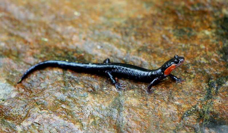
For the analysis, I will only use widely publically available data sets. As for a species, I’ve chosen the very charasmatic Jordan’s Red Cheeked Salamander, endemic to the Great Smoky Mountains National Park (USA).

For this tutorial, you’re going to need the following libraries installed:

• gdistance
• tidyverse
• rgeos
• elevatr
• ggplot2
• tigris
• spocc
• raster
• viridis
• ggthemes

To save space and reduce the amount of intermediate variables, I will make use of the tidyverse syntax. This includes using data processing features of dplyr as well as pipes (%>%). If you prefer not to use these features, simply focus on the key functions and data sources which can easily be incorporated into your own preferred work flow.

Let’s get started!

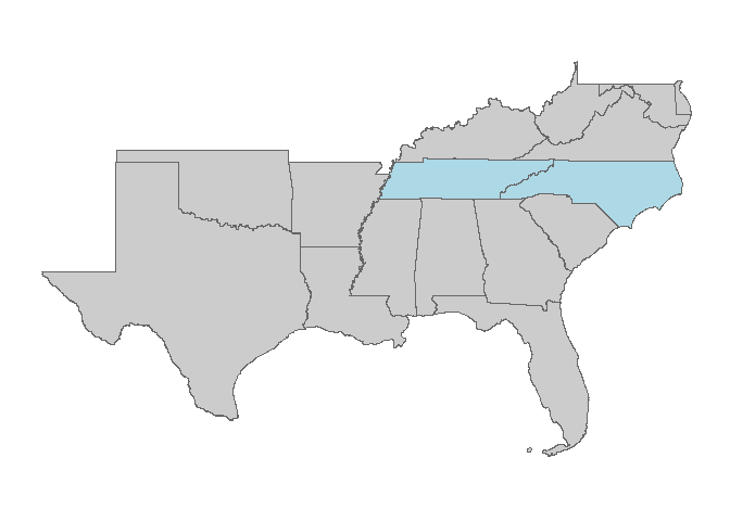
First, lets download a shapefile to work with.

library(tigris)         # Tigris package for USA census data
library(tidyverse)
states <- states()

se <- states %>%
  subset(REGION == "3") 

TN_NC <- se %>%     # Subsetting the data to Tennessee and North Carolina
  subset(NAME %in% c("Tennessee", "North Carolina"))

Next, lets download some species occurrence records for Jordan’s Red Cheeked Salamander (JRCS) from the Global Biodiversity Information Facility using the R package spocc. In this query, I will pull only the first 1000 records. Yes, that means I’m pulling records in no particular order, and that they can be biased. Don’t @ me.

library(spocc)

## Warning: package 'spocc' was built under R version 4.0.2

library(raster)

## Warning: package 'raster' was built under R version 4.0.2

## Loading required package: sp

## 
## Attaching package: 'raster'

## The following object is masked from 'package:dplyr':
## 
##     select

## The following object is masked from 'package:tidyr':
## 
##     extract

Pj <- occ(query = "Plethodon jordani",                 # JRCS scientific name
          from = "gbif",                               # limiting query to *the first* 1000 records
          limit=1000,                                  # limiting query to *the first* 1000 records
          has_coords = T)                              # limiting those 1000 records to those that have geo-referenced data

Now that we have the data, we need to organize and clean it using dplyr. Luckily, spocc has improved their naming system, so this is easier to do now.

Pj_sp <- Pj$gbif$data$Plethodon_jordani %>%            # Grabbing the Darwin-core data from the spocc object
  dplyr::select(longitude,                             # Keep locations and year, discard the rest
                latitude,
                year) %>%                   
  dplyr::filter(year > 2000) %>%                       # Filter records to only those after year 2000
  filter(!duplicated(round(longitude, 2),              # Remove duplicate records using rounded decimals (this removes points very near to one-another)       
                     round(latitude, 2)) == TRUE) %>%  # >> See notes below about ^^
  dplyr::mutate(lon = scale(longitude),                # Remove points far outside the cluster of occurrences
                lat = scale(latitude)) %>%             # >> See notes below about ^^
  dplyr::filter(!abs(lon)>2) %>%
  dplyr::filter(!abs(lat)>2) %>%
  dplyr::select(longitude,
                latitude) %>%
  SpatialPoints(proj4string = crs(se)) 

Notes To remove stacked points, or points that are clustered very closely, I rounded the decimal points to the second hundreths place and removed duplicates. This step is actually very biologically meaningful… Because we want to map potential flow between populations of JRCS, we want each point to represent a population–meaning each point must be sufficiently isolated so as to only be connected through stochastic disperal. Because JRCS is dispersal limited, I chose to remove points less that ~10 km from one another (approximately the resolution of the second decimal point of a gps coordinate).

I removed points that were suspiciously far outside the cluster of presences by creating new variables: lon and lat, which are Z-scores of the latitude and longitude variables (by subtracting the mean and dividing by standard deviation, or using the scale function). I them removed values greater that 2, which represent points that are two standard deviations from the mean latitude and mean longitude.

Let’s plot our points

library(ggplot2)
library(viridis)

## Loading required package: viridisLite

library(ggthemes)

ggplot() + geom_polygon(data=se, aes(x=long, y=lat, grou=group), col="grey40", fill="grey80") +
  geom_polygon(data=TN_NC, aes(x=long, y=lat), col="grey40", fill="light blue") + 
  coord_quickmap() + theme_map()

## Regions defined for each Polygons

## Warning: Ignoring unknown aesthetics: grou

## Regions defined for each Polygons

To create a custom study area, shaped to our occurrence points, we can create a convex hull around our points using chull().

Pj_coords <- Pj_sp@coords                                                  
Pj_chull <- chull(Pj_sp@coords)                           # Creating convex hull

Pj_chull_ends <- Pj_sp@coords[c(Pj_chull, Pj_chull[1]),]  # generate the end points of polygon. 
Pj_poly <- SpatialPolygons(
  list(Polygons(
    list(Polygon(Pj_chull_ends)), ID=1)),
                             proj4string = crs(se))       # convert coords to SpatialPolygons 

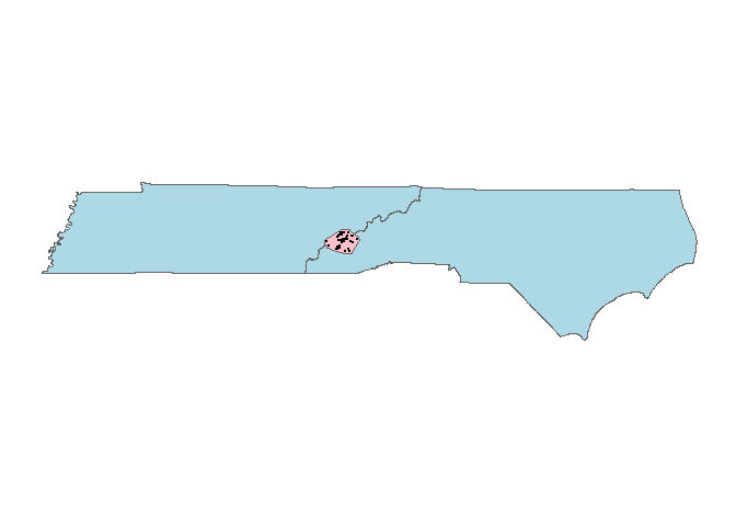
Now, we will create a buffer around those points using rgeos::gBuffer().

library(rgeos)
Pj_poly_buff <- gBuffer(Pj_poly, width = 0.05, byid=T)

Let’s have a look at your buffered polygon:

ggplot() + geom_polygon(data=TN_NC, aes(x=long, y=lat), col="grey40", fill="light blue") + 
  geom_polygon(data=Pj_poly_buff, aes(x=long, y=lat, grou=group), col="grey40", fill="pink") +
  geom_point(data=as.data.frame(Pj_sp@coords), aes(x=longitude, y=latitude), size=0.01) + 
  coord_quickmap() + theme_map()

## Regions defined for each Polygons

## Warning: Ignoring unknown aesthetics: grou

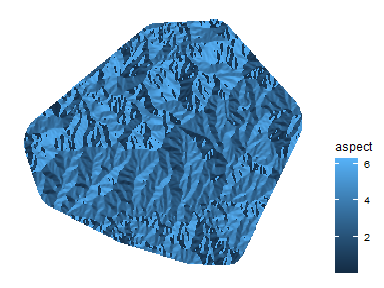
To create our resistance layers for the connectivity analysis, let’s download a digital elevation model (DEM) using package elevatr.

library(elevatr)
elevation <- get_elev_raster(Pj_poly_buff, z = 8)         # This will find a DEM tile nearest to our polygon 

While elevation is important, we can derive other biologically important variables using the raster::terrain(), inlcuding aspect (direction a hillside is facing) and topographic roughness index (TRI). In very simple terms, TRI calculates the change in elevation between a point and its surroundings (in a neighborhood of 8 points).

elv <- elevation %>%                                      # First, lets cut the DEM to our study area 
  crop(Pj_poly_buff) %>%                                  # crop to the extent
  mask(Pj_poly_buff)                                      # mask to the edges

asp <- terrain(elv, opt="aspect", neighbors = 8)          # Calculate aspect

ggplot(as.data.frame(asp, xy=T)) + geom_raster(aes(x=x, y=y, fill=aspect)) + 
  scale_fill_continuous(na.value=NA) + theme_map() + theme(legend.position = "right")

## Warning: Removed 18361 rows containing missing values (geom_raster).

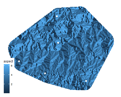
To simplify our analysis for this demonstration, I’m going to cut down the number of presence points to only 5. Because we will be calculating pairwise random shortest-paths (from now on, “random walks”), we will calculate 10 paths.

set.seed(6)                                               # To make your results match mine
Pj_sample <- Pj_coords[sample(nrow(Pj_coords), 5),]       # Take 5 random locations

ggplot(as.data.frame(asp, xy=T)) + geom_raster(aes(x=x, y=y, fill=aspect)) + 
  geom_point(data=as.data.frame(Pj_sample), aes(x=longitude, y=latitude), size=2, col="white") +
  scale_fill_continuous(na.value=NA) + theme_map()

## Warning: Removed 18361 rows containing missing values (geom_raster).

To make our pairwise random walks, we have to create a side index. Here’s quick little solution I made which creates a matrix of every conceivable combination of points:

Pj_combn <- combn(nrow(Pj_sample),2) %>%
  t() %>%
  as.matrix()

To perform a random walks analysis, we have to create a transition matrix using gdistance::transition(), as well as perform a geocorrection.

library(gdistance)
asp_tr <- transition(asp, transitionFunction = mean, 4) %>%
    geoCorrection(type="c",multpl=F)

Now comes the fun part. This loop will perform the random walk routine using gdistance:passage() for each pairwise path, generating a flow map. This flow map can be considered as “conductance” a la Circuitscape, or the “probabilities of passages” based on randomized shortest-paths.

passages <- list()                                                     # Create a list to store the passage probability rasters in
system.time(                                                           # Keep track of how long this takes
  for (i in 1:nrow(Pj_combn)) {           
    locations <- SpatialPoints(rbind(Pj_sample[Pj_combn[i,1],1:2],     # create origin points
                                      Pj_sample[Pj_combn[i,2],1:2]),   # create destination (or goal) points, to traverse
                                crs(se))
    passages[[i]] <- passage(asp_tr,                                   # run the passage function 
                                  origin=locations[1],                 # set orgin point
                                  goal=locations[2],                   # set goal point
                             theta = 0.00001)                             # set theta (tuning parameter, see notes below)
    print(paste((i/nrow(Pj_combn))*100, "% complete"))
  }
)

## [1] "10 % complete"
## [1] "20 % complete"
## [1] "30 % complete"
## [1] "40 % complete"
## [1] "50 % complete"
## [1] "60 % complete"
## [1] "70 % complete"
## [1] "80 % complete"
## [1] "90 % complete"
## [1] "100 % complete"

##    user  system elapsed 
##   15.89    2.88   18.76

passages <- stack(passages)                                            # create a raster stack of all the passage probabilities
passages_overlay <- sum(passages)/nrow(Pj_combn)                       # calculate average

Notes In our passage function, we set theta, (θ), a tuning parameter. Extremely low values result in a random walk (equivilant to Circuit Theory), but as θ¸ increases, the passage converges on least cost path. I supplied a value somewhere in the middle.

colors <- c("grey60", viridis_pal(option="plasma", begin = 0.3, end = 1)(20))
ggplot(as.data.frame(passages_overlay, xy=T)) + geom_raster(aes(x=x,y=y,fill=layer)) +
  scale_fill_gradientn(colors = colors, na.value = NA) + 
  theme_map() +   theme(legend.position = "right")

## Warning: Removed 18361 rows containing missing values (geom_raster).

There you have it!

Now, this was an extremely short demonstration… In the future, I plan to make many additional posts on connectivity, what it means, how to use it, as well as provide some more tutorials.

Best,

-Alex.