Machine Learning the 'Tidy' Way
A tutorial on K-nearest neighbor and boosted trees using the tidymodels framework
Introduction to machine learning with tidymodels
Tidymodels provides a clean, organized, and–most importantly–consistent programming syntax for data pre-processing, model specification, model fitting, model evaluation, and prediction.
Anatomy of tidymodels
a meta-package that installs and load the core packages listed below that you need for modeling and machine learning
rsamples: provides infrastructure for efficient data splitting and resampling
parsnip: a tidy, unified interface to models that can be used to try a range of models without getting bogged down in the syntactical minutiae of the underlying packages
recipes: a tidy interface to data pre-processing tools for feature engineering
workflows: workflows bundle your pre-processing, modeling, and post-processing together
tune: helps you optimize the hyperparameters of your model and pre-processing steps
yardstick: measures the effectiveness of models using performance metrics
dials: contains tools to create and manage values of tuning parameters and is designed to integrate well with the parsnip package
broom: summarizes key information about models in tidy tibble()s
First, lets load the tidymodels meta-package:
library(tidymodels)
library(tidyverse)
Package tutorials:
Data
I’ll demonstrate it’s features using an existing data set from Bruno Oliveria, Amphibio:
- Link to publication: https://www.nature.com/articles/sdata2017123
- Link to data: https://ndownloader.figstatic.com/files/8828578
Amphibio data
Download data:
# install.packages("downloader")
# library(downloader)
#
# url <- "https://ndownloader.figstatic.com/files/8828578"
# download(url, dest="dial_broom/amphibio.zip", mode="wb")
# unzip("dial_broom/amphibio.zip", exdir = "./dial_broom")

library(readr)

amphibio_raw <- read_csv("AmphiBIO_v1.csv")
The data consist of natural history information of amphibians, including habitat types, diet, size, ect.
Here’s the breakdown of taxonomic spread in the data:
- Order: N = 3
- Family: N = 61
- Genera: N = 531
- Species: N = 6776
There are also a lot of missing data, and what data do exist are wildly different scales. We’ll clean this up:
# Check how many NA's for each row
amphibio <- amphibio_raw %>%
  select("Order"
         ,"Body_mass_g"
         ,"Body_size_mm"
         ,"Litter_size_min_n"
         ,"Litter_size_max_n"
         ,"Reproductive_output_y"
         ) %>%
  na.omit %>%
  mutate(Body_mass_g = log(Body_mass_g),
         Body_size_mm = log(Body_size_mm),
         Litter_size_min_n = log(Litter_size_min_n),
         Litter_size_max_n = log(Litter_size_max_n),
         Reproductive_output_y = log(Reproductive_output_y)) %>%
  filter(!Order == "Gymnophiona")

amphibio %>%
  group_by(Order) %>%
  summarize(n = n())
Now let’s have a peak at the data:
  amphibio %>%
  pivot_longer(!Order, names_to = "Metric", values_to = "Value") %>%
  ggplot(aes(Order, Value, col = Order)) +
    geom_boxplot() +
    facet_wrap(~Metric)
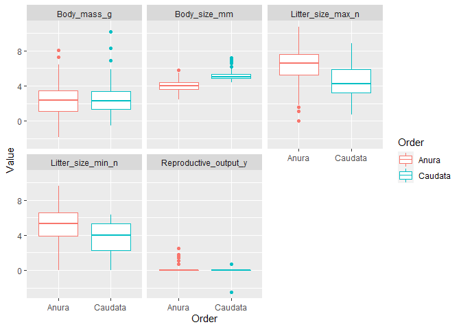
There are some trends in the data:
- caudates are longer
- anura have larger litter sizes
Given the data, one possible modeling application could be to use data to predict order using two models: knn and boosted regression trees.
To start the modeling process, we’ll use rsamples to split the data
into training and testing sets.
set.seed(42)

tidy_split <- initial_split(amphibio, prop = 0.95)
tidy_train <- training(tidy_split)
tidy_test <- testing(tidy_split)
tidy_kfolds <- vfold_cv(tidy_train)
We can use recipes to preprocess the data:
# Recipes package
## For preprocessing, feature engineering, and feature elimination
tidy_rec <- recipe(Order ~ ., data = tidy_train) %>%
  step_dummy(all_nominal(), -all_outcomes()) %>%
  step_normalize(all_predictors()) %>%
  prep()
Now that we’ve created a recipe to process the data for modeling, we can
use parsnip to model the data:
First, let’s have a look at the model’s description
library("webshot")
# ?boost_tree
boost_tree()
Description
boost_tree() defines a model that creates a series of decision trees
forming an ensemble. Each tree depends on the results of previous trees.
All trees in the ensemble are combined to produce a final prediction.
There are different ways to fit this model. See the engine-specific pages for more details:
xgboost (default)
C5.0
spark
?nearest_neighbors
nearest_neighbor():
defines a model that uses the K most similar data points from the training set to predict new samples.
There are different ways to fit this model. See the engine-specific pages for more details:
- knn (default)
Now, let’s fit the models:
# Parsnip package
## Standardized api for creating models
tidy_boosted_model <- boost_tree(trees = tune(),
                                min_n = tune(),
                                learn_rate = tune()) %>%
  set_mode("classification") %>%
  set_engine("xgboost")

tidy_knn_model <- nearest_neighbor(neighbors = tune()) %>%
  set_mode("classification") %>%
  set_engine("kknn")
Our basic model recipe is complete, but now we want to use dials to
tune parameters.
dials
For boosted regression trees, there are 3 basic parameters:
parameters(tidy_boosted_model)

## Collection of 3 parameters for tuning
##
##  identifier       type    object
##       trees      trees nparam[+]
##       min_n      min_n nparam[+]
##  learn_rate learn_rate nparam[+]
trees: An integer for the number of trees contained in the ensemble.min_n: An integer for the minimum number of data points in a node that is required for the node to be split further.learn_rate: A number for the rate at which the boosting algorithm adapts from iteration-to-iteration (specific engines only).
Knn has a single parameter to tune: the neighbors
parameters(tidy_knn_model)

## Collection of 1 parameters for tuning
##
##  identifier      type    object
##   neighbors neighbors nparam[+]
neighbors: A single integer for the number of neighbors to consider (often called k). For kknn, a value of 5 is used if neighbors is not specified.
So, we can use dials to set the possible parameter values, which can
then be tuned using tune.
# Dials creates the parameter grids
# Tune applies the parameter grid to the models
# Dials pacakge
boosted_params <- 5
knn_params <- 10

?grid_regular

## starting httpd help server ... done

boosted_grid <- grid_regular(parameters(tidy_boosted_model), levels = boosted_params)
boosted_grid

## # A tibble: 125 x 3
##    trees min_n   learn_rate
##    <int> <int>        <dbl>
##  1     1     2 0.0000000001
##  2   500     2 0.0000000001
##  3  1000     2 0.0000000001
##  4  1500     2 0.0000000001
##  5  2000     2 0.0000000001
##  6     1    11 0.0000000001
##  7   500    11 0.0000000001
##  8  1000    11 0.0000000001
##  9  1500    11 0.0000000001
## 10  2000    11 0.0000000001
## # ... with 115 more rows

knn_grid <- grid_regular(parameters(tidy_knn_model), levels = knn_params)
knn_grid

## # A tibble: 10 x 1
##    neighbors
##        <int>
##  1         1
##  2         2
##  3         4
##  4         5
##  5         7
##  6         8
##  7        10
##  8        11
##  9        13
## 10        15
Implement tuning grid using tune:
tune
# install.packages(c("xgboost", "kknn"))
library(xgboost)
library(kknn)

# Tune pacakge
# system.time(
#   boosted_tune <- tune_grid(tidy_boosted_model,
#                             tidy_rec,
#                             resamples = tidy_kfolds,
#                             grid = boosted_grid)
# )
# write_rds(boosted_tune, "boosted_tune.rds")
boosted_tune <- read_rds("boosted_tune.rds")

# system.time(
#   knn_tune <- tune_grid(tidy_knn_model,
#                         tidy_rec,
#                         resamples = tidy_kfolds,
#                         grid = knn_grid)
# )
# write_rds(knn_tune, "knn_tune.rds")
knn_tune <- read_rds("knn_tune.rds")

#Use Tune package to extract best parameters using ROC_AUC handtill
boosted_param <- boosted_tune %>% select_best("roc_auc")
knn_param <- knn_tune %>% select_best("roc_auc")
#Apply parameters to the models
tidy_boosted_model_final <- finalize_model(tidy_boosted_model, boosted_param)
tidy_knn_model_final <- finalize_model(tidy_knn_model, knn_param)
Now, well try different options from dials for parameter tuning, using
two additional methods for grid specification:
- random grid with
dials::grid_random - maximum entropy grid with
dials::grid_max_entropy
grid_random
boosted_grid_rand <- grid_random(parameters(tidy_boosted_model), size = boosted_params)
boosted_grid_rand

## # A tibble: 5 x 3
##   trees min_n learn_rate
##   <int> <int>      <dbl>
## 1   190    21   2.32e- 5
## 2  1816    12   3.60e- 8
## 3   293    28   3.14e-10
## 4   314     8   2.52e- 7
## 5  1363     5   5.92e- 6

knn_grid_rand <- grid_random(parameters(tidy_knn_model), size = knn_params)
knn_grid_rand

## # A tibble: 7 x 1
##   neighbors
##       <int>
## 1         1
## 2        10
## 3         5
## 4         3
## 5        11
## 6         8
## 7         2

# system.time(
#   boosted_tune_rand <- tune_grid(tidy_boosted_model,
#                                  tidy_rec,
#                                  resamples = tidy_kfolds,
#                                  grid = boosted_grid_rand)
# )
# write_rds(boosted_tune_rand, "boosted_tune_rand.rds")
boosted_tune_rand <- read_rds("boosted_tune_rand.rds")

# system.time(
#   knn_tune_rand <- tune_grid(tidy_knn_model,
#                              tidy_rec,
#                              resamples = tidy_kfolds,
#                              grid = knn_grid_rand)
# )
# write_rds(knn_tune_rand, "knn_tune_rand.rds")
knn_tune_rand <- read_rds("knn_tune_rand.rds")

#Use Tune package to extract best parameters using ROC_AUC handtill
boosted_param_rand <- boosted_tune_rand %>% select_best("roc_auc")
knn_param_rand <- knn_tune_rand %>% select_best("roc_auc")
grid_max_entropy
boosted_grid_maxent <- grid_max_entropy(parameters(tidy_boosted_model), size = boosted_params)
boosted_grid_maxent

## # A tibble: 5 x 3
##   trees min_n learn_rate
##   <int> <int>      <dbl>
## 1   433    25   4.27e-10
## 2  1671    13   3.28e-10
## 3  1520     3   3.21e- 6
## 4   672     3   3.06e-10
## 5  1371    22   2.32e- 5

knn_grid_maxent <- grid_max_entropy(parameters(tidy_knn_model), size = knn_params)
knn_grid_maxent

## # A tibble: 10 x 1
##    neighbors
##        <int>
##  1         3
##  2        10
##  3         1
##  4        15
##  5        13
##  6         4
##  7         6
##  8         8
##  9         9
## 10        11

# system.time(
#   boosted_tune_maxent <- tune_grid(tidy_boosted_model,
#                                    tidy_rec,
#                                    resamples = tidy_kfolds,
#                                    grid = boosted_grid_maxent)
# )
# write_rds(boosted_tune_maxent, "boosted_tune_maxent.rds")
boosted_tune_maxent <- read_rds("boosted_tune_maxent.rds")

# system.time(
#   knn_tune_maxent <- tune_grid(tidy_knn_model,
#                                tidy_rec,
#                                resamples = tidy_kfolds,
#                                grid = knn_grid_maxent)
# )
# write_rds(knn_tune_maxent, "knn_tune_maxent.rds")
knn_tune_maxent <- read_rds("knn_tune.rds")

#Use Tune package to extract best parameters using ROC_AUC handtill
boosted_param_maxent <- boosted_tune_maxent %>% select_best("roc_auc")
knn_param_maxent <- knn_tune_maxent %>% select_best("roc_auc")
workflows
For combining model, parameters, and preprocessing
boosted_wf <- workflow() %>%
  add_model(tidy_boosted_model_final) %>%
  add_recipe(tidy_rec)

knn_wf <- workflow() %>%
  add_model(tidy_knn_model_final) %>%
  add_recipe(tidy_rec)
yardstick
For extracting metrics from the model
boosted_res <- last_fit(boosted_wf, tidy_split)
knn_res <- last_fit(knn_wf, tidy_split)
mods <- bind_rows(
boosted_res %>% mutate(model = "xgb"),
knn_res %>% mutate(model = "knn")) %>%
unnest(.metrics)
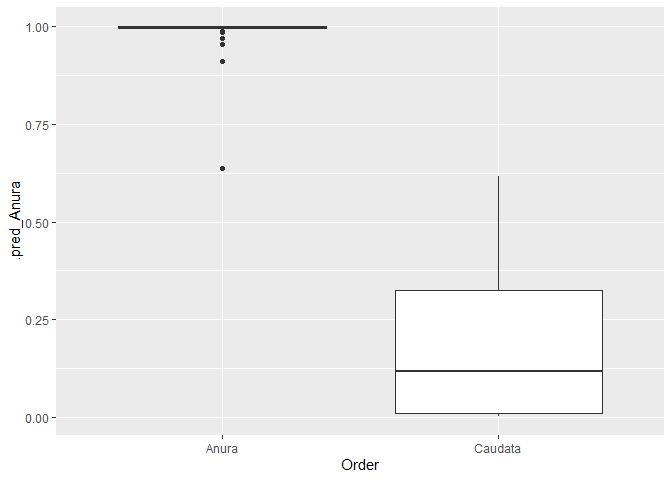
ggplot(bind_rows(mods$.predictions), aes(Order, .pred_Anura)) +
geom_boxplot()
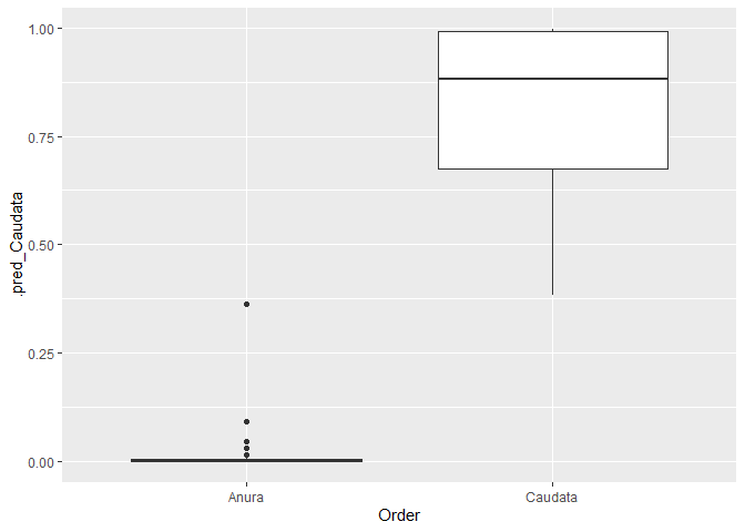
ggplot(bind_rows(mods$.predictions), aes(Order, .pred_Caudata)) +
  geom_boxplot()
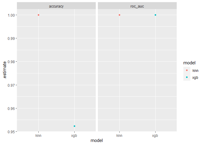
ggplot(mods, aes(x = model, y = .estimate, col = model)) +
  geom_point() +
  facet_wrap(~.metric)
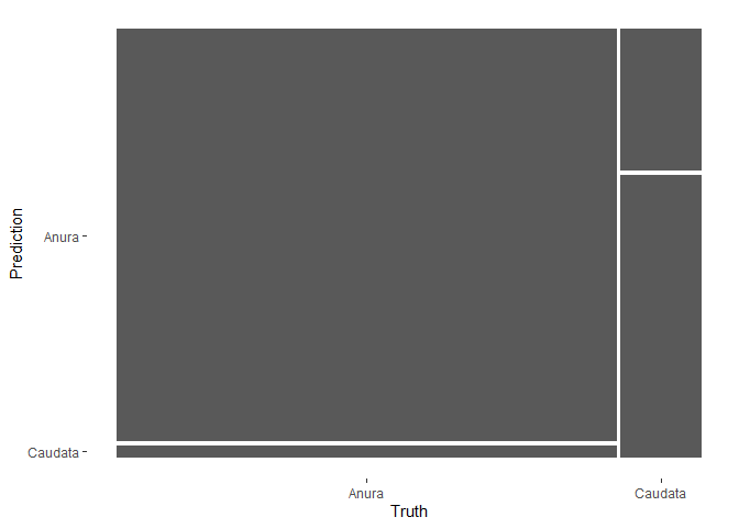
Confusion matrix to visualize model predictions against truth
boosted_res %>% unnest(.predictions) %>%
  conf_mat(truth = Order, estimate = .pred_class) %>%
  autoplot()
Fit the entire data set using the final wf
final_boosted_model <- fit(boosted_wf, amphibio)

## [15:25:37] WARNING: amalgamation/../src/learner.cc:1095: Starting in XGBoost 1.3.0, the default evaluation metric used with the objective 'binary:logistic' was changed from 'error' to 'logloss'. Explicitly set eval_metric if you'd like to restore the old behavior.

final_knn_model <- fit(knn_wf, amphibio)
broom
Now we can use broom to tidy the results from these models, and
provide an intuitive view of their meaning!
augment()
First, we’ll use augment to obtain predictions, residuals, and other
items from the model, which auto-binds them to the original dataset.
boosted_aug <- augment(final_boosted_model, new_data = amphibio[,-1])
knn_aug <- augment(final_knn_model, new_data = amphibio[,-1])

boosted_aug_long <- boosted_aug %>%
  pivot_longer(-c(.pred_class, .pred_Anura, .pred_Caudata), names_to = "predictor", values_to = "value")
Now we can evaluate the models using yardstick!
yardstick
final_boosted_model %>%
predict(bake(tidy_rec, new_data = tidy_test), type = "prob") %>%
bind_cols(tidy_test) %>%
roc_auc(factor(Order), .pred_Anura)
## # A tibble: 1 x 3
## .metric .estimator .estimate
## <chr> <chr> <dbl>
## 1 roc_auc binary 0.759
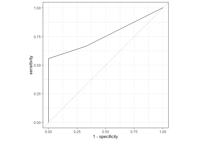
final_boosted_model %>%
predict(bake(tidy_rec, new_data = tidy_test), type = "prob") %>%
bind_cols(tidy_test) %>%
roc_curve(factor(Order), .pred_Anura) %>%
autoplot()
Evaluating knn model
final_knn_model %>%
predict(bake(tidy_rec, new_data = tidy_test), type = "prob") %>%
bind_cols(tidy_test) %>%
roc_auc(factor(Order), .pred_Anura)
## # A tibble: 1 x 3
## .metric .estimator .estimate
## <chr> <chr> <dbl>
## 1 roc_auc binary 0.5
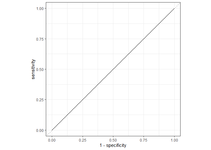
final_knn_model %>%
predict(bake(tidy_rec, new_data = tidy_test), type = "prob") %>%
bind_cols(tidy_test) %>%
roc_curve(factor(Order), .pred_Anura) %>%
autoplot()
final_knn_model %>%
  predict(bake(tidy_rec, new_data = tidy_test), type = "prob") %>%
  bind_cols(tidy_test) %>%
  roc_auc(factor(Order), .pred_Anura)

## # A tibble: 1 x 3
##   .metric .estimator .estimate
##   <chr>   <chr>          <dbl>
## 1 roc_auc binary           0.5
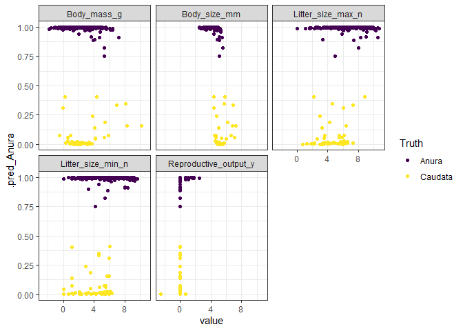
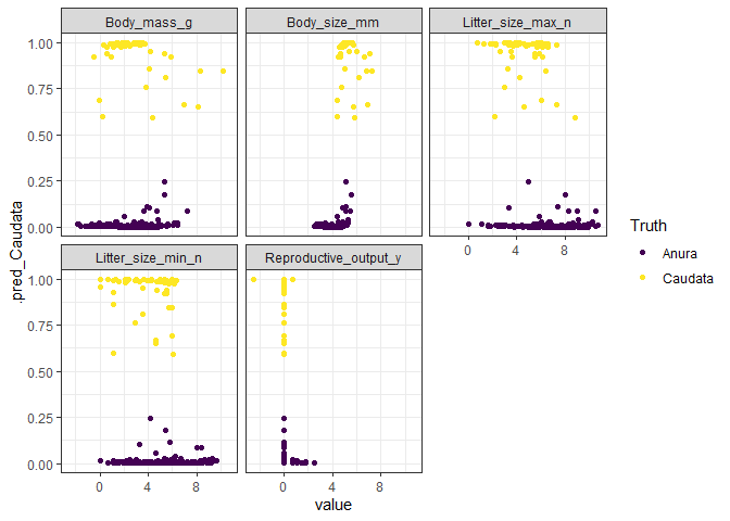
Visualizing predictions:
library(viridis)

## Loading required package: viridisLite

##
## Attaching package: 'viridis'

## The following object is masked from 'package:scales':
##
##     viridis_pal

ggplot(boosted_aug_long, aes(x = value, y = .pred_Anura, col = .pred_class)) +
  geom_point() +
  facet_wrap(~predictor) +
  scale_color_viridis_d("Truth", option = "D") +
  theme_bw()
ggplot(boosted_aug_long, aes(x = value, y = .pred_Caudata, col = .pred_class)) +
  geom_point() +
  facet_wrap(~predictor) +
  scale_color_viridis_d("Truth", option = "D") +
  theme_bw()
J Alex Baecher
Postdoctoral Researcher
My research interests include landscape ecology and applied conservation of reptiles and amphibians